Arthur A. Few Wednesday, November 12, 2003

I think this exercise is a great learning device for the undergraduate students. In addition to the obvious computer skills that are learned, consider the important scientific principles involved in this exercise and the associated reading in the text.

1. The Conservation of Energy & 1st Law of Thermodynamics
2. The Transformation of Energy: Light - Heat - Infrared
3. Heat Capacity & Temperature
4. Albedo, Solar Constant, Effective Planetary Temperatures
5. The Blackbody Radiation Law
6. Kirchoff’s Law: Absorptivity = Emissivity
7. The Greenhouse Principle
8. The Role of the Oceans in Climate
9. System Behavior: Time Constants, Feedback, Initial Conditions,
Asymptotic Approach to Equilibrium, Steady State
10. And, The Human Input of Atmospheric CO₂ will produce global warming


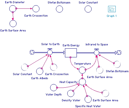
Part 1. Creating a Working Model with STELLA^®II
Create your own model for the Earth energy system described in Section V, Building Working Models: The Earth Energy System. Print a copy of your system diagram, your equations, and your graphic results to submit as part of your assignment.
The exercise should be done in units of years, and DT should be of the order of 0.01 year; Euler’s method is sufficient. Using a time unit of a year requires that we convert all physical parameters (i.e., Solar constant & Stefan-Boltzmann constant) from units containing seconds to years. (One day is 86,400 s, and one average year is 31,557,600 s, which includes the leap-year effect.)

© 1992, Arthur A. Few. All rights reserved.

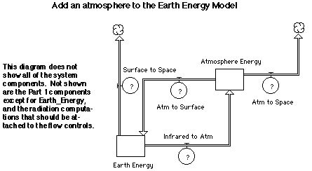
Part 2. Add a One-Layer Atmosphere.
The basic Earth energy model created in Part 1 will be modified by adding an atmospheric layer with radiative properties similar to our atmosphere (i.e. transparent to visible and absorbing in the infrared). The atmospheric parameters will be adjusted to achieve a global temperature appropriate for the Earth.
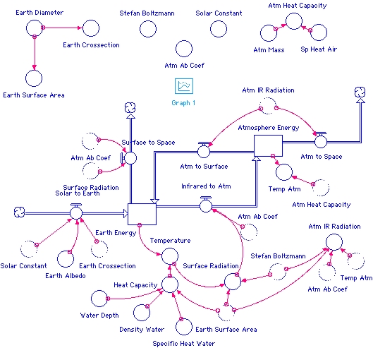
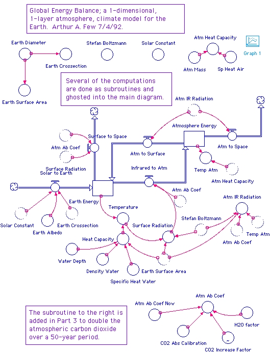
Make a copy of your model from Part 1 (Duplicate or Save As), and modify it by adding the Atmosphere Energy reservoir and infrared energy flows shown below (Infrared to Space has been replaced by the components shown below). Change the Water Depth to 100 m (the mixing depth for the oceans). It will now have the appropriate time constant relative to the atmosphere. This also allows for larger time steps (~0.1 year), but requires running the model for 100 years to reach equlibrium.

When you examine the Infrared to Space equation in Part 1 you will notice that it is the black-body radiant flux, (area)*sT⁴. The atmosphere is not a black body, but we may use a “gray body” approximation for the atmosphere in which the radiant flux from the atmosphere is given by (Atmos Ab Coef)*(area)*sT⁴. (This is Kirchhoff’s Law.) In this expression Atmos Ab Coef is the atmospheric absorption coefficient, a number between zero and one. The atmosphere radiates equally upward and downward. The fraction of the Earth surface radiation absorbed by the atmosphere is determined by Atmos Ab Coef, and the fraction of the Earth surface radiation that passes through the the atmosphere to space is (1 - Atmos Ab Coef).
You will also need the following information to complete the model:
The mass of the atmosphere, Mass Atmos = 5.14e18 kg.
Specific heat of air, Sp Ht Air = 1004 J/kg K.
Change the depth of the water in the Earth surface, Water Depth = 100 m.
Simulation Time settings: Experiment with these values. The model exhibits strange behavior with dt = 1.0 years because the time step is larger than the atmospheric time constant. Try it, and watch the atmospheric temperature.
Computation Method = Euler’s.
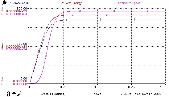
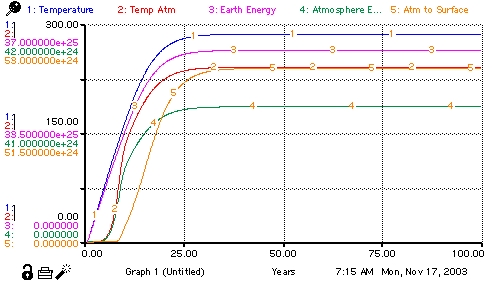
The parameter “Atmos Ab Coef” is our unknown in Part 2. We know from Part 1 that without an atmosphere the surface temperature of the Earth is 255 K. The mean temperature of the Earth’s surface is now approximately 288 K ~ 15 C. You should, using the technique of trial and error correction, find the value of Atmos Ab Coef which produces an Earth surface temperature of 288 K. Make a list of your trials and results. Print a copy of your system diagram, your equations, and your graphic results to submit as part of your assignment. You may print the graphic results of each trial or just print your final trial on which you write the results of your previous trials. You must submit the answers to your trials.
You should record the values of the Earth Energy and Atmospheric Energy from Part 2 to use as the initial values for Earth Energy and Atmospheric Energy in Part 3; you can eliminate or reduce the warm-up period of the Earth climate model.


Part 3. Explore the Effect of Doubling Atmospheric CO₂.
We are going to modify the model of Part 2 to explore the effect of doubling atmospheric CO₂ over a 50-year time span. Make a copy of your model from Part 2 for use here. Insert the initial conditions saved from Part 2 in the reservoirs. Create a new converter and name it Atm Ab Coef Now, and give it the value that you found for Atm Ab Coef in Part 2. This is the starting value for Part 3.
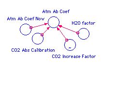
Add the components shown to the right to your system diagram. Atm Ab Coef becomes a variable in Part 3.
We need to develop a relationship between a , Atm Ab Coef, and the changing concentration of carbon dioxide, which is controlled by the multiplier, CO2 Increase Factor, which ranges from 1 to 2. I have not found a source for a in the literature because we are treating the whole atmosphere as a single layer. We will develop the needed relationship from empirical data and GCM m

odel results. I will give you the results of my evaluation here and provide the details in the footnote.
a₀ = Atm Ab Coef Now, b = CO2 Abs Calibration, f = CO2 Increase Factor, and w = H2O factor. The estimate is: a = a₀ + w * b * (f - 1) .
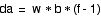
The increase in a is a linear function of the increase in the fractional carbon dioxide concentration
(f - 1). w is a multiplier for the water-vapor feedback, and b is the constant of proportionality determined by comparison with GCM model output. The values for these parameters can be found in the footnote. You will find that w is given over a range of values; choose a value near the middle of this range for the first model run.
The converter – CO2 Increase Factor – is a graphic variable that specifies the changes in CO2 Increase Factor over time. The ~ in the converter identifies it as a graphical converter. The figure below shows how your graphic variable should look.

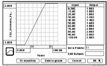
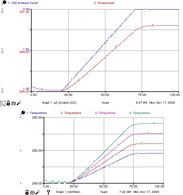
We allow 20 years for the system to re-equilibrate since our initial conditions were not precise to many decimal places. The carbon dioxide doubles linearly over 50 years. And, we allow another 30 years for the system to reach a new steady state. This is a 100-year model run.
Run your model and display CO2 Increase Factor and Temperature; print this result. Why is there a lag between the carbon dioxide change and the temperature response? Write your answer to this question on the printed graphic.
Now that your model is working we will use the sensitivity-study capabilities of STELLA to compare the temperature outputs for 4 values of H2O Factor, w, over the range 1.5 to 3.0. The sensitivity dialog box is accessed from the Run Menu as Sensi Specs…; here you will specify the number of comparative model runs and the range of w. Print a copy of your system diagram, your equations, and your sensitivity runs graphic results to submit as part of your assignment.


Comment.
Having completed the modeling exercise you see the necessity of including an atmosphere in order to model the climate system. However, a 1-layer atmosphere has serious limitations. For example, the maximum greenhouse warming obtainable (a = 1) is , which for the Earth would be 303 K or an increase of 48 K. We are at 33 K now, which is not far from the limit. The greenhouse warming for Venus is ~500 K, an impossible task for a 1-layer atmosphere.
The more layers that are used to model the atmosphere the better the approximation. Each layer can have a smaller absorption coefficient and the perturbations are smaller. Every layer and the surface must communicate by radiation with all of the others. A multi-layer model has lots of plumbing!


Footnote.
A survey article, “Climate Modelers Struggle to Understand Global Warming,” (Physics Today, February, 1990, 17-19) provides some of the information that we need for this exercise.
Exercises 1 & 2 at the end of Section V of the System Behavior and System Modeling develop much of the analytical descriptions of the global energy balance model in the steady state, and the Instructor’s Manual elaborates these solutions. The sensitivity equation for the atmospheric absorption coefficient (p.37 in SB&SM and p. 18 &19 in IM) is

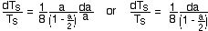
When integrated these equations give

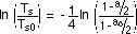
We can verify the consistency of the two approaches to the problem by inserting the following values into this last equation: T_s0 = 255 K, T_s = 288 K, a₀ = 0. The solution for a is 0.77, which is exactly the result from Part 2. For small changes in warming the differential form of these equations should be accurate. We can verify this by setting T_s0 = 288 K and a₀ = 0.77 for today’s values and letting dT_s = 2 K, which is in the bounds described in the attached reading for global warming. Both the integral and differential forms yield the same result for a (=0.804), accurate to the third significant figure. We can confidently use the differential forms for global warming studies.

The differential form of the equation becomes: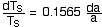

The absorption coefficient, a, represents all of the greenhouse gases. We will separate it into two terms; a_c for carbon dioxide and a_w for water vapor, but a_w actually represents all of the other greenhouse gases. Hence, da = da_c + da_w . The attached reading says that including the water vapor term increases the dT by a factor, w, in the range 1.5 to 3.0. We can, therefore write two equations, where the “c” denotes the contribution of carbon dioxide alone.

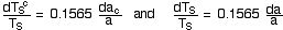
The ratio of the second to the first of these equations yields

where w is the H2O factor in the range 1.5 to 3.0 obtained from the reading. We are somewhat closer to the answer but not yet there. We have from above da = w * da_c , and we now seek relationship between da_c and carbon dioxide concentration, C , where the present value is C₀. Since most small perturbations follow a linear relationship we will assume the following form for da_c. (Doubling, however, is not a small perturbation.)

where b is a constant to be determined empirically. Combining the results from the last four equations we find

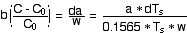
For a doubling of carbon dioxide (C - C₀)/ C₀ = 2, dT_s = 1.5 K to 4.5 K, and w = 1.5 to 3.0;
thus b = 0.0171 to 0.02563. We will assume, therefore, that b = 0.02, the CO2 Abs Calibration. Our empirical estimate is

where f is the CO2 factor, i.e., C = f * C₀ . This last equation is the one that we use in the model calculations.

#