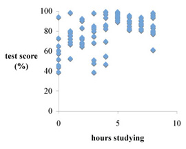
poor correlation
good correlation
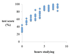
Typically, we use a scatter plot of raw data for a rather specific purpose, namely when we want to know how well two variables are correlated. For example, you might want to know if student scores on a final exam are directly related to the number of hours that students claimed to have studied. Highly scattered data may suggest a poor correlation, while very "tight" data usually suggest good correlation.
poor correlation
|
good correlation
|
When we are interested in presenting trends rather than a correlation, we usually simplify things by converting the data to useful summary values. Our scatter plot of raw data shows that there is some correlation between time and height. Given the investigator's interest in representing the central tendency of each sample, perhaps it would be a good idea to convert the data after all.
Your plot will be simplified if you convert each week's measurements into a single useful number that represents the central tendency of the data set. What sort of conversion should you use?
Plot high/low values
Plot a mean (average value) for each week
Plot a median (middle number in the list) for each week
Plot the mode (most common value) for each week
Time is the independent variable, to be plotted on the x axis; height (a measured quantity) is a dependent variable, to be plotted on the y axis.
Because time and height are continuous parametric variables, the logical choice for plotting them is a scatter plot (XY scatter).
Column graphs (vertical) are often used in a scientific context, but they are for categorical, not continuous, variables.
Some data plotting software will disguise a line graph as a plot for two continuous variables, but actually treats the independent variable as categorical.
Horizontal bar, pie, doughnut, line, area, 3D and other "exotic" plot types are seldom used in a scientific context.
Weekly height measurements for seedlings of Acer palmatum:
| week | 0 | 2 | 4 | 6 | 8 | 10 | 12 |
| measured | 1.2 | 1.4 | 1.4 | 1.9 | 5.8 | 5.7 | 5.3 |
| heights | 0.3 | 0.5 | 2.0 | 3.0 | 2.9 | 4.8 | 5.1 |
| in inches | 1.1 | 1.0 | 2.3 | 3.8 | 4.9 | 4.8 | 8.5 |
| 1.1 | 1.7 | 2.2 | 2.6 | 3.7 | 8.2 | 8.2 | |
| 1.0 | 1.8 | 2.4 | 3.5 | 5.6 | 6.1 | 7.0 | |
| 1.5 | 2.2 | 2.0 | 2.3 | 4.8 | 4.8 | 5.5 | |
| 1.3 | 1.5 | 2.0 | 3.1 | 1.1 | 8.3 | 5.6 | |
| 0.8 | 1.5 | 2.1 | 3.1 | 4.6 | 6.1 | 2.2 | |
| 1.7 | 1.7 | 2.5 | 4.3 | 4.2 | 7.4 | 4.8 | |
| 1.5 | 1.6 | 1.6 | 5.0 | 5.1 | 3.7 | 8.4 | |
| 1.6 | 1.2 | 2.7 | 1.8 | 3.8 | 4.3 | 4.3 | |
| 1.1 | 1.2 | 1.5 | 2.8 | 7.4 | 4.3 | 5.9 |
NOTE: You may wish to copy the entire table at this point and paste the data into cell B1 of a blank Excel spreadsheet