Reviews in Undergraduate Research - Issue 2

SUMMARY

Molecular dynamics (MD) is a widely used tool in condensed matter physics, as well as other disciplines ranging from chemistry to high-energy physics. In MD, one integrates the equations of motion - Newton's second law for classical particles - directly, invoking no approximations. To do so requires an interaction potential energy or forces between atoms. I will discuss both integration schemes and potential types. MD potentially bridges two length scales - macroscopic and atomistic - and also links experimental results with theories. This will be emphasized through a discussion of modern research in solid-state physics, with each research application highlighting a different type of interaction potential. I will discuss fluid flow briefly and highlight some other applications of Lennard-Jones potentials, surface growth using a Stillinger-Weber potential, and defects in silicon using tight-binding potentials. I give some references regarding density-functional theory calculations of these defects.

A different avenue of modern MD research is in the method itself rather than its application. Much research is towards developing so-called acceleration methods. By taking advantage of the physics of condensed matter systems, acceleration methods have been proposed which extend the time scales accessible by MD by orders-of-magnitude in many cases. In this article, I will focus on A. F. Voter's methods, giving their motivation, algorithm, and some derivations.

In short, this article explain why MD is useful and where it has been used, it gives the fundamentals necessary for understanding a MD simulation, and discusses research into MD methods themselves, namely Voter et al.'s acceleration methods.

INTRODUCTION

Molecular dynamics (MD) is a widely used tool in condensed matter physics, as well as other disciplines ranging from chemistry (Kityk et al., 1999) to high-energy physics (Bleicher et al., 1999). This article focuses on applications to solid-state physics; however, the basic concepts presented should be valuable to any newcomer to MD, regardless of their field.

One of MD's appeals is that the system in consideration is simulated directly - without assuming the nature of transitions or the types of the structures. Moreover, due to increasing computer power, MD provides atomistic detail for system sizes that are exponentially increasing to mesoscopic scales. Already, with classical potentials, simulations are performed with hundreds of millions of atoms for hundreds of picoseconds (Kadau et al, 2002) or with a more accurate tight-binding potential simulating about 64 atoms for 0.250 microseconds (Richie et al., 2002) - nearly a timescale measurable on a stopwatch!

Note that MD bridges two scales - macroscopic and atomistic - and thus links experimental results, say transport measurements, with theories governing the interactions of the simulated matter's constituent atoms. Indeed, conventional "pencil-and-paper" theory generally cannot evaluate the properties that are of direct consequence in experiments. In this light, MD forms another bridge, one between experiments and conventional theory. By iterating the process of performing simulations and experiments, theories of forces between atoms are refined.

With MD now appropriately evangelized, the exposition of the fundamentals begins. Traditional (non-accelerated) MD is conceptually simple. Using some potential interaction between particles, Newton's second law updates the particles' velocities and positions; repeating this, the equations of motion are integrated and the system's trajectories are obtained. In order to be relevant at finite temperature, pressure, etc., the system must be modified to ensure it stays at a constant energy, temperature or in whichever thermodynamic ensemble is desired. Methods of simulating the correct ensemble are not given here but can be found in (Rapaport, 1997).

Before giving specific examples of research into new MD methods (acceleration methods), I present the more technical aspects of MD. Expositions of integration algorithms follow a background in potentials. Accelerating MD motivates the parallel-replica, hyperdynamics, and temperature-accelerated dynamics acceleration methods, as well as on-the-fly kinetic Monte Carlo. Finally, illustrative research at the forefront of MD simulation in solid-state physics is discussed; each piece of research highlights a different class of potentials.

POTENTIALS

To accurately propagate the system, we must have an accurate interaction potential. This potential gives the potential energy as a function of the atomic positions and velocities. Details on existing potentials are given, as well as some general ways of deducing potentials.

Common Potentials

One can generally group potentials into three basic categories: classical potentials, tight-binding potentials, and density-functional calculations, in order of increasing computational complexity. Representative examples are discussed: Lennard-Jones (LJ), MEAM, and Stillinger-Weber (SW); empirical tight-binding (TB); and density-functional theory (DFT). LJ considers interactions between pairs of atoms; MEAM adds corrections, beyond pairwise interactions, based on the local geometry; TB and DFT add quantum mechanics at increasingly sophisticated levels. Each potential will be discussed later in terms of a particular research application.

Regardless of the potential, deriving its form requires assumptions, or the form of the potential may just be guessed. In optimizing a potential's accuracy, parameters are adjusted (like the balance between attractive and repulsive LJ parameters - see below) so the potential reproduces quantities such as lattice constants and defect energies obtained from first-principles calculations or experiment (Baskes, 2001).

Efficient Potential Calculations - see (Rapaport, 1997) for more information

Once the potential is obtained, it must be computed repeatedly in a MD simulation, a O(N²) or worse calculation, where N is the number of particles, rendering simulation of large systems impossible. A O(N) calculation is achieved in practice by one of two methods:

1. The "cell method" - This method divides the system being simulated into cells, each with a linear size larger than the interaction cutoff r_c (Figure 1), where r_c is a value such that atoms farther apart than this value essentially do not interact. Now one needs only to compute interactions between atoms in the same and adjacent cells (Figure 1), causing a speedup to O(N) for even moderate size systems.

2. The "neighbor list method" -- In fact, only 16% of the atoms, on average, included in the cell method are within a distance of r_c (Rapaport, 1997). Hence we keep a list of all "neighbors" of an atom. This is actually an O(N²) calculation. Fortunately, one can code this efficiently and only compute it only once every many time-steps since there is an upper bound to how fast things are moving, effectively making the overall system an efficient O(N) calculation for most system sizes.

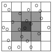Figure 1. Two-dimensional illustration of the cell method. The dark gray cell needs only to check the light gray cells – its nearest neighbors – because all other atoms must lie outside of the interaction cutoff range rc, the range beyond which no particles interact.

 

POSITION INTEGRATION ALGORITHMS

Some details of potentials and their calculation are now familiar. With the potential and initial conditions Newton's second law can be integrated for all the particles. The verlet and predictor-corrector (PC) methods are common for performing the integration.

The integration algorithm usually does not need to be extremely accurate. Because an extremely slight position displacement at any time (or an equivalent round-off error) can cause huge differences in the atom's trajectory at all later times after a certain time, only quantities which are insensitive to exact trajectories "matter." This is not particular to MD, but is characteristic of the natural process itself.

The verlet method gives positions at a short time t after the time corresponding to the supplied positions. Each is derived in a straightforward manner from the Taylor expansion, in time, of the atomic coordinates. The formula for the verlet propagator is (Rapaport, 1997) .

The verlet propagator is commonly used for its simplicity and tendency to conserve energy.

The PC methods are more accurate than verlet, but they are not used as frequently as the simpler verlet-class propagators. The primary advantage of the PC method over the verlet-like algorithms is in the ability to change Δt on the fly, which may be useful in systems where one set of particles inherently move faster than others. PC is also useful when constraints (on, say, bond length or angles) are placed on the system (Rapaport, 1997).

The PC method predicts positions based upon Adams-Bashforth extrapolation, which is exact if they follow monic polynomials. After prediction, correction is made via a different set of formulae. For the (relatively complex) equations see (Rapaport, 1997).

BETTER (FASTER!) MOLECULAR DYNAMICS

Although MD is an increasingly mature field, there are still continuous advances in methods. Voter et al. have developed several methods for increasing MD's performance by many orders of magnitude. Each method requires some assumptions - usually forms of transition state theory (TST) (Voter, 2002 or Lombardo, 1991) - on the nature of transitions. However, the assumptions are minimal and their validity can be checked.

There are three common families of acceleration techniques, namely parallel-replica (PR or par-rep), temperature-accelerated dynamics (TAD), and hyperdynamics. The families can be utilized simultaneously for multiplicative performance boosts. Voter gives an excellent, accessible review concentrating on these acceleration methods (Voter, 2002).

The limitation that keeps one from simulating long time scales is the fact that MD is a multi-scale problem (for most solid-state systems). Specifically, one must use a small enough integration time step to reproduce the dynamics of the fast vibrational modes. Since these vibrations occur on the order of 10¹³ - 10¹⁴ times a second, the time step for accurate integration must be on the order of femtoseconds. A typical time step falls in the range of 1-5 fs.

On the other hand, transitions occur infrequently; time scales between interesting transitions range from picoseconds (quickly diffusing surface atoms) to seconds (dislocation motion under shearing (Haasen, 1996)). One can conceive of watching interesting behavior for minutes or hours (for example, in crystal growth), however the longest MD simulations can now run for only microseconds. It must be kept in mind that the acceleration methods discussed below only apply to infrequent event systems, systems in which the time for transitions between 'sites' or 'structures' is much longer than the vibrational period.

Parallel Replica

When running MD simulations on parallel computers such as clusters one can separate the calculation so that each processor deals only with a portion of the atoms. Thus increasing the number of processors one can increase the size of the simulated system. However, each processor must have many atoms associated to it or else the communication time between processors, rather than the computational time, will be the performance bottleneck. While a spatial decomposition of the problem is conceptually easy, there is no straightforward way to decompose the simulation in time because each set of positions requires the previous positions.

To solve this problem, Voter created the parallel-replica (PR) algorithm (Voter, 1998). The only assumption of PR is that the probability of a system escaping a site (transitioning from one potential minimum to another) between times t and t+dt is given by

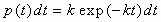Eqn. 1

 

where k is the rate constant.

This is satisfied by infrequent systems when the sites are uncorrelated (Voter, 2002). Here uncorrelated means that once a system enters a new potential well (crosses a saddle point in the potential energy surface) it has no "memory" of the site it just arrived from; that is, the dynamics after the crossing are not affected by how it got to that site.

The PR method has been extended to work when the probability distribution function has a different form than Eq. 3 (Shirts, 2001). However, one must be very careful in this case as it indicates that a "state" is composed of several potential minima or that the runs on each processor are not independent (see below).
With this assumption, the parallel-replica procedure can be shown to give the same dynamics as a system simulated with non-accelerated dynamics in the sense that the sequences of transitions from state to state are reproduced in the long time limit. I will present how the procedure works; for a proof, see (Voter, 2002).

To start a parallel-replica simulation, identical systems are set up on multiple processors. The number of processors can often be very large and consist of many different types/speeds of processors. Now, to ensure that each processor is simulating independent trajectories, the dynamics run at finite temperature with momenta randomized every few time steps.

All the processors now run dynamics until the system on one of the processors escapes from its current state. The time elapsed on each processor is summed and this is identified as the total time spent in the state from which the system has just escaped. The processor that computed the escape continues to run for a certain length of time such that after this additional time there is no memory of the state from which the system escaped.

The PR method solves, to some degree, the process of parallelizing MD in the time domain. It has been often utilized (Zagrovic B, 2001; Shirts, 2000; or Birner, 2001). Still, much the performance of the individual processors can be increased. Hyperdynamics and temperature-accelerated dynamics are two solutions to this problem and are discussed next.

Hyperdynamics

One (justified) way to view the time evolution of a system is as a succession of vibrational and transitional 'events'. This is illustrated in Figure 2; the system oscillates in this potential well for a certain time, and then an increase in local energy pushes the system over the transition barrier to a new potential well (Figure 2a). Remember that this is a high-dimensional potential well; forgetting this can misguide intuition.

Using this picture of dynamics, one can imagine speeding up the simulation by "filling in" the wells (Figure 2b). However, to do this one must be able to decide (automatically) whether the system is close to the bottom of the well or near the transition point, since the potential should be filled in more or less, respectively. Even assuming that one can fill in the wells with some technique, one must map the dynamics of the boosted system back to the non-accelerated systems. Voter et al. describes this process in (Voter, 2002).

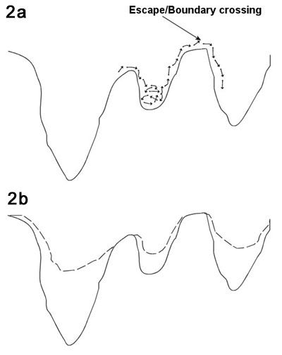Figure 2. Viewing dynamics as a sequence of vibrational and translational events – applicable to many condensed matter systems – and the relation to hyperdynamics. a. The particle oscillates in its potential minimum then the energy of the system is temporarily increased, pushing the system over an energy barrier. b. By decreasing the depth of the potential wells, the dynamics are sped up since less energy is required to cross the barrier.

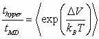
As a last note, the average boost factor for hyperdynamics is given by

with Boltzmann's constant, T the temperature, and the increase in potential energy from the bias potential. This implies that we receive an exponentially bigger boost as the temperature of interest lowers. Hyperdynamics has not found nearly as much success as other acceleration methods due to technical difficulties in filling in the potential wells.

Temperature-accelerated Dynamics

The temperature-accelerated dynamics (TAD) method has been more successful than hyperdynamics to date. This method is related to hyperdynamics in that one increases transition frequencies by making the energy barriers easier to go over. Rather than changing the relative energetics, however, TAD simply raises the temperature of the system.

As with hyperdynamics, the accelerated dynamics will not directly correspond to the non-accelerated dynamics; rather, by some a priori assumptions, the dynamics are mapped to the lower (correct) temperature dynamics. In place of a usual MD simulation, basin-constrained MD (BCMD) is performed in which the system is evolved until a transition occurs. After this is detected, the trajectory is reversed, sending the system back into the basin from which it had just escaped. The saddle point is calculated using, say, the nudged-elastic band method (Henkelman, 2000) and stored. This continues until a specified certainty is reached that one possesses enough information to properly extrapolate the dynamics to lower temperature.

Harmonic transition-state theory (HTST) - the assumption placed on the system in this method - states that the probability distribution for first escape times for the basin in consideration is given by Eq. 1, with

Eq. 2

 

 

where E_a is the energy barrier the system must go over to escape from the basin, and v₀ is some frequency characterizing how often the system vibrates or attempts to leave the basin (the attempt prefactor).

Note that these equations explain why raising the temperature changes the dynamics; changing the temperature does not affect merely the magnitudes of each rate constant, but affect also the relative magnitudes (hence speed up one transition more than another). To extrapolate the transition time from high to low temperature

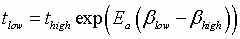Eqn. 3

 

 

is used (Figure 3), where t_low is the time at the low temperature and t_high is the time at the high temperature; , and E_a is the activation energy computed by nudged-elastic band or a related method (Henkelman, 2000).

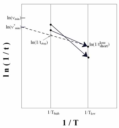Figure 3. Temperature-accelerated dynamics in a picture. The system runs at high temperature until it escapes from a potential minima and the time is then extrapolated to low temperature. After being reflected back into the potential basin, the simulation runs to time tstop at which point the extrapolated low-temperature time is correct with a specified certainty.

 

To derive Eq. 3, change variables in the probability distribution (Eq. 1) to . Then . Hence has the same probability distribution as , and .

This relation is illustrated graphically in Figure 3. Here it is clear that a transition that is not the shortest at high temperatures can be the shortest at a lower temperature - this is why basin-constrained dynamics must be performed. The transition with the shortest time for escape (at low temperature) is selected as the transition corresponding to the low-temperature dynamics and the system is updated. 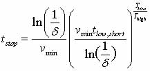The BCMD is started again from this new site. To be confident, with certainty δ, that the current shortest time t₀ (at low-temperature T_low) is correct, the system must run in BCMD for a time

where v_min is the minimum attempt prefactor (see Eq. 2) which can be chosen manually, using reasonable guesses; t_low,short is the shortest found time (extrapolated to low-temperature) (Voter, 2002).

Using this technique, one boosts the simulation speed by a factor of hundreds when interested in low enough temperature systems (a couple hundred Kelvin). Recently, Voter proposed a TAD enhancement (Montalenti, 2001) in which one considers the total time spent in a state (previous and current visit). This requires a good way of telling if two states are the same, within symmetry, a topic just being explored in condensed matter systems (Jiang, 2003 and Machiraju, 2003). With this improved TAD method, the average boost factor for each state becomes

with E_min the minimum barrier for escape from the state in consideration (Montalenti, 2001).

I briefly mention on-the-fly kinetic Monte Carlo (OTF-KMC) simulations. KMC uses a user-specified list of transition rates and, by sampling from the rate list, propagates the system in time. KMC requires a priori knowledge of the transitions and their rates, which is problematic. OTFKMC computes the list of transitions by MD simulation (Voter, 2002) or other means (Henkelman, 2003) as the simulation progresses. When the system returns to a state enough times, one assumes that the rate list is nearly complete and uses KMC. To see applications of TAD and OTFKMC, see (Sprague, 2002 or Montalenti, 2002 or Montalenti, 2001).

RECENT SIMULATIONS

Lenard-Jones Potential: Fluid Flow and Biophysics

Now I focus on current simulations performed using MD, starting with Lennard-Jones (LJ) potentials. LJ potentials are pairwise interaction potentials. That is, the total potential energy of a system is just a sum over all possible pairs i,j of atoms of a potential energy function , where U is a function only of relative atomic positions of two atoms. These interactions capture the essence of many systems, and produce quantitatively the behavior of noble gas (say argon) liquids and gases in many cases - the noble gases were historically very important for the LJ potential (Collings, 1971, for example).

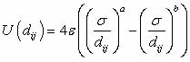
In the LJ potential there are two parameters: one parameter governs the strength of the attractive interaction and one of the repulsive interaction; equivalently one can use a parameter as the potential minima depth, and another as the atomic separation for the potential minimum (σ and ε respectively below). The basic formula for calculating the (LJ a-b) potential is

Usually a=12 and b=6; if this is the case the potential is generally just denoted LJ (rather than LJ 12-6). In Figure 4 one can see the strong repulsive core at short ranges and the weak attractive tail. The a=12 parameter is fairly arbitrary (fortunately some physics is relatively insensitive to the choice of a) and the value of b=6 comes from Van der Walls attraction of non-polar substances.

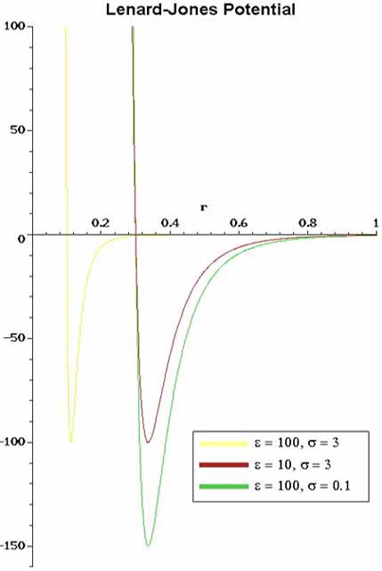Figure 4. The usual Lennard-Jones (LJ 12-6) interaction potential. The graph is potential energy as a function of interatomic distance.

In addition to the noble gases, the LJ potential is still used as part of the total potential in biological applications (Schleyer, 1998 or Brooks, 1983). In these situations, long-range interactions are Coulombic and LJ, and short-range interactions (bonded atoms) obey Hooke's law. In testing new methods, low dimensional LJ model systems are often used. These systems have the advantage of giving qualitatively complicated and atomic-like potential surfaces as well as, in some cases, being analytically solvable. This, coupled with the quickness of their simulation, gives rise to LJ's usefulness in testing models.

Moreover, the potentials occasionally find use in condensed matter outside of biophysics. Despite the extreme simplicity of this model, it shows many complex phenomena characteristic of condensed matter systems (phase transitions, complex energy landscapes, infrequent events) and hence is studied to see the simplest examples of these phenomena (Scopigno, 2002 and Fabricius, 2002). A systematic study of large numbers of clusters of particles interacting via LJ yields interesting results on the dynamics and structures of these clusters, while suggesting general features that hint at features in real clusters (Doye, 1999). Also, when extremely large numbers of particles need to be simulated yet a continuum approach is not applicable, such as in some fluid flow problems, LJ is attractive. Millions of particles can be simulated for many time steps.

As an example, Berthier and Barrat (Berthier, 2002) have studied mixtures of sheared fluids using a LJ potential. Two types of particles are implemented via particle-type dependent σ's and ε's in the LJ potential. They are able to investigate velocity distributions, viscosity dependence on shear rate, and structure factors for the system at different temperature, spanning liquid, supercooled, and glassy states. Hence, they investigate this macroscopic system at an atomistic level of detail, bridging these length scales as promised in the introduction. They also correlate theoretical predictions (using a "mode-coupling approach") with the simulations, demonstrating another of the bridges discussed at the start. Others have used LJ to study fluid flow as well - for a flavor, try (Bruin, 1998 or Laredji, 1996).

Classical Potentials (beyond Lenard-Jones)

The LJ potential does not include how the environment (nearby atoms) affects the pairwise interaction. That is, the potential depends on terms involving three or more relative positions, but LJ ignores this. Extra terms are necessary to accurately simulate many systems.

Typical potentials that incorporate these many-body interactions (in very different ways) are modifications to LJ to include explicit angular dependence, Stillinger-Weber (SW) (Stillinger, 1985), and the modified embedded atom method (MEAM) (Daw, 1984). Recently, MEAM has been used to tackle a large variety of systems; largely these have been surface diffusion/surface growth phenomena.

Lee et al. (Lee, 1998) and (Baskes 1997) (and many others) have studied ad-dimer (two atoms deposited on top of a surface) diffusion on silicon surfaces. Adatom (one deposited atom) diffusion was studied earlier (Roland, 1992). Here I will describe results garnered by Gawlinski and Gunton (G&G) for molecular-beam epitaxial (MBE) growth of Si(001) surfaces (Gawlinski, 1987), a simulation which involves diffusion of adatoms and ad-dimers as well as coalescence: the clusters meet and 'stick,' forming islands. G&G employed a SW potential for the simulation.

Some investigations have looked at the detailed mechanisms of the diffusion of these small clusters and coalescence of these. G&G chose to discuss only the morphology (basic shape) of the surfaces grown and to not discuss the exact mechanisms, since classical potentials may not properly incorporate important effects.

In MBE, atoms are deposited (in this case as single atoms) from the gas phase onto the crystal surface. G&G were inspired to simulate this process, in part, by the experimental discovery of an epitaxial growth transition temperature. Above this temperature the atoms, after striking the surface, have time to diffuse around and find globally stable (bulk-like) states; below this temperature, however, new atoms are deposited close to already deposited atoms before the deposited atoms can relax. This leads to amorphous (no local order) surface grown on the bulk phase (Gawlinski, 1987). One of the simulation goals was predicting this transition temperature; they succeeded in finding a temperature in good agreement with theory (Gawlinski, 1987).

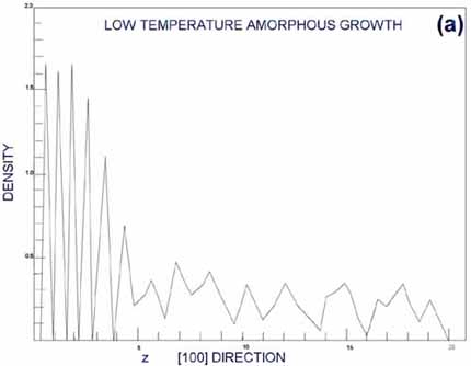
In an ordered, layered crystal structure, the density of atoms as a function of some coordinate should have oscillatory behavior with sharp peaks. In amorphous structures, the density should be spread out relatively smoothly. Figures from G&G (Gawlinsky, 1987) are reproduced as Figures 5a,b. Figure 5a is the density of deposition occurring above the epitaxial transition temperature; Figure 5b is the corresponding density below the epitaxial transition temperature. Clearly, the top layers represented in Figure 5a are well layered, and in Figure 5b they seem more random. This case forms an excellent example of MD forming the third bridge I mentioned in the introduction, that with experiment.

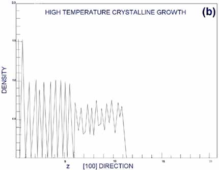Figure 5. Density of atoms as a function of depth from surface. From (Gawlinski, 1987). a. Periodic peaks in the density profile indicate a well-ordered, layered crystal structure. This occurs above the epitaxial growth temperature, when individual atoms have time to relax to bulk-like states before new atoms restrict their movement. b. A smoother density profile at the surface indicated amorphous surface growth, occurring below the epitaxial growth temperature.

While it is possible to compare simulation results with experiment, one must be extremely cautious in several regards. First, a simulation is only as accurate as the potentials used, leading to the cautious interpretation above (no detailed mechanisms). Moreover, in order to run this simulation (in 1987, even!) the deposition rate of incoming atoms had to be increased to extremely unrealistic values. If the time between atomic depositions should match experiment, it is likely that no depositions would have occurred in the time scale simulated. With this is mind, however, something must be going correctly, or the simulation would not have reproduced experiment.

Tight-binding Potentials and Density Functional Theory

While purely classical potentials have worked extremely well in some situations, often quantum effects are important. Both tight-binding (TB) and density-functional theory (DFT) methods incorporate quantum mechanical effects at some level. TB incorporates these at a much less accurate level than DFT, but TB is a couple orders-of-magnitude faster to calculate. Moreover, TB can scale linearly with system size in some cases by exploiting the fact that the calculation is essentially diagonalizing a sparse matrix (Galli, 1998 or Klimeck, 2002). DFT is also widespread in the literature, including the problem of silicon defect clusters discussed below (for example, Kohyama, 1999; Estreicher, 1998; or Windl, 1999). I focus on TB.

TB has found use in cluster and defect structure and defect diffusion in some materials (Arai, 1997 or Jansen, 1988). In particular, it has been used to simulate interstitial (extra atoms inserted between lattice sites) and vacancy (atom removed from lattice site) clusters. Also, groups have studied more extended structures such as the {311} defect in silicon (Kim, 2000). This is by no means an exhaustive list.

Many studies of defect clusters in silicon are not MD simulations, but only energetic calculations, especially in DFT. In investigations such as these, initial structures are guessed and then the system is locally minimized (Estreicher, 1998). The downside to this is the guessing. Quite un-intuitive structures are typical (Richie, 2002) and missed by simple guessing. A few people (Wilkins, private communication) are advocates of performing "cheap" TB or classical MD to explore a problem and improve guesses for structures and transition pathways, followed by DFT energy calculations to confirm results.

Colombo reviews TB results of silicon defects in (Colombo, 2002). Naively, it may seem that when an interstitial meets a vacancy, they should annihilate, leaving only bulk silicon. This state is energetically favored, and, if given an infinite amount of time, the system will spend most of its time in the bulk state. However, experiments and experience tend to deal with finite time scales on the order of seconds. Tang et al., (Tang, 1997) find that if an interstitial and a vacancy are placed within next nearest neighbors along the <110> direction (in which the dimer points) then annihilation does occur. If the vacancy and interstitial are instead separated by greater than next nearest neighbors they do not annihilate; they attract each other and form a stable interstitial-vacancy pair shown in Figure 6. The energy barrier for annihilation once achieving this state is greater than 1 eV, corresponding to a lifetime of hours for the defect at room temperature. This strange structure is a concrete example of why guessing structures and interaction mechanisms can fail (Richie, 2002 or Kim, 2000).

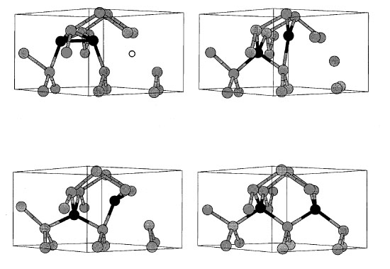Figure 6. A stable interstitial-vacancy cluster (one extra atom, one missing atom) and its annhilation path. This unintuitive structure (top left) is higher in energy than its lowest energy state (perfectly crystalline), but there is a very large energy barrier between the two states. At room temperature such interstitial-vacancy clusters are stable for hours.

As a final note on this research, note that I have artificially assigned each problem domain to a type of potential. Often, these problems do not use the potential types I suggest. For example, hydrogen atoms effect on Si(001) surfaces have been studied with DFT (Dongxue, 2002); classical potentials have been used to study Si clusters (Birner, 2001); and TB potentials have been used for Ge diffusion on Si (110) surfaces (Katircioglu, 1994). The applications I have presented are a small fraction of all simulations performed - there is little limit to MD's applications thanks to the lack of assumptions on the dynamics.

CONCLUSIONS

This review does not cover all classes of research using MD - references are representative rather than exhaustive. However, it should have given the reader an idea of some typical applications - fluid dynamics, surface growth, and defect dynamics. Through examples, connections between experiment, theory, and MD are emphasized. One now hopefully has a feeling for the variety and advantages of some potential types.

Also one should now be aware of some of the growing number of molecular dynamics acceleration methods - parallel-replica, temperature-accelerated dynamics, hyperdynamics, and on-the-fly Monte Carlo. Perhaps the most important information presented is the necessary background to understand what goes into an MD simulation. With this and the references, a motivated individual could probably code a simplistic MD simulator in a matter of a week (though given the increasing number of sophisticated, fast MD programs, writing one from scratch is probably not advisable except as a teaching tool).

ABOUT THE AUTHOR

Kaden Hazzard is a third-year undergraduate at The Ohio State University planning on graduating in the spring of 2004. He plans on pursuing a doctoral degree in condensed matter physics. He intends to pursue a research career at a university or at a national lab. He has been involved in computational condensed matter physics with Professor John Wilkins's research group since the summer of 2000. He has been researching a variety of topics, mainly defect evolution in silicon; surface growth in silicon; and structure recognition, characterization, and data mining of defects in solids. He has implemented several routines in the group's multi-scale materials simulator (OHMMS), and a new Monte Carlo method for calculating free energies. He also spent the summer of 2002 at Los Alamos National Labs doing low-temperature experimental work.

ACKNOWLEDGEMENTS

Everyone in Professor John Wilkin's research group who I have had the fortune to work with deserves thanks for their continued guidance, discussions, and ideas. In particular, I would like to thank Professor Wilkins for his continuous suggestions for improving this manuscript and my writing in general. I would also like to thank Angela K. Hartsock for her gracious help with the figures.

FURTHER READING

(Rapaport, 2002) is the standard for general aspects of MD and (Voter, 2002) gives an excellent review of acceleration methods.

A standard text regarding MD in general, along with many techniques especially for simulations of liquids is
Allen, M.P., Tildesley, D.J. (1989) Computer Simulation of Liquids

For those interested in finding out more about density-functional theory, a preprint for a good review article accessible to undergraduates who have taken some quantum mechanics, I suggest:
Capelle, K. (2003) A bird's-eye view of density-functional theory cond-mat/0211443

REFERENCES

Arai, N., Takeda , S., and Kohyama, M. (1997) Self-Interstitial Clustering in Crystalline Silicon Physical Review Letters 78 4265

Baskes, M.I. (1997) Calculation of the behaviour of Si ad-dimers on Si(001) Modelling Simul. Mater. Sci. Eng. 5 p. 149-158.

Berthier, L. and Barrat, J.L. (2002) Shearing a Glassy Material: Numerical Tests of Nonequilibrium Mode-Coupling Approaches and Experimental Proposals Physical Review Letters 89 95702

Birner, S., Kim, J., Richie, D.A., Wilkins, J.W., Voter, A.F., and Lenosky, T. (2001) Accelerated dynamics simulations of interstitial-cluster growth. Solid State Communications 120 (7-8)

Bleicher, M., Zabrodin, E., Spieles, C., Bass, S.A., Ernst, C., Soff, S., Bravina, L., Belkacem, M., Weber, H., Stöcker, H., and Greiner, W. (1999) Relativistic Hadron-Hadron Collisions in the Ultra-Relativistic Quantum Molecular Dynamics Model (UrQMD) J.Phys. G25 1859-1896

Brooks, B. R., Bruccoleri, R. E., Olafson, B. D., States, D. J., Swaminathan, S., and Karplus, M. (1983) CHARMM: A Program for Macromolecular Energy, Minimization, and Dynamics Calculations. J. Comp. Chem. 4, 187-217

Bruin, C. (1998) Wetting and drying of a rigid substrate under variation of the microscopic details Physica A vol. 251, issues 1-2, pp 81-94

Chen, D. and Boland, J. J. (2002) Chemisorption-induced disruption of surface electronic structure: Hydrogen adsorption on the Si(100)-2x1 surface Physical Review B (Condensed Matter and Materials Physics). vol.65, no.16 15. p. 165336/1-5.

Collings, A.F., Watts, R.O., and Woolf, L.A. (1971) Thermodynamic properties and self-diffusion coefficients of simple liquids. vol.20, no.6 p. 1121-33.

Colombo, L. (2002) Tight-binding theory of native point defects in silicon. Annu. Rev. Mater. Res., Vol. 32: 271-295

Daw, M.S. and Baskes, M.I. (1984) Embedded-atom method: Derivation and application to impurities, surfaces, and other defects in metals. Phys. Rev. B 29, 6443

Doye, J.P.K., Miller, M.A., and Wales, D.J. (1999) Evolution of the Potential Energy Surface with Size for Lennard-Jones Clusters. , J. Chem. Phys. 111, 8417-8428

Estreicher, S. K., Hastings, J. L., and Fedders, P. A. (1999) Hydrogen-defect interactions in Si. Materials Science & Engineering B (Solid-State Materials for Advanced Technology) E-MRS 1998 Spring Meeting, Symposium A: Defects in Silicon: Hydrogen v 58 n 1-2 p.31-5

Fabricius, G. and Stariolo, D.A. (2002) Distance between inherent structures and the influence of saddles on approaching the mode coupling transition in a simple glass former. Phys. Rev. E 66, 031501

Galli, G., Kim, J., Canning, A., and Haerle, R. (1998) Large scale quantum simulations using Tight-Binding Hamiltonians and linear scaling methods Tight-Binding Approach to Computational Materials Science, Eds. P. Turchi, A. Gonis and L. Colombo, 425 (1998).

Gawlinski, E.T. and Gunton, J.D. (1987) Molecular-dynamics simulation of molecular-beam epitaxial growth of the silicon (100) surface. Phys. Rev. B 36, 4774-4781

Haasen, Peter. (1996) Physical Metallurgy. (Cambridge University Press) pp. 282-283

Henkelman, G., Jóhannesson, G., and Jónsson, H. (2000) Methods for Finding Saddle Points and Minimum Energy Paths, Progress on Theoretical Chemistry and Physics, Kluwer Academic Publishers, Ed. S. D. Schwartz and references therein.

Henkelman, G. and Jónsson, H. (2003), Multiple time scale simulations of metal crystal growth reveal importance of multi-atom surface processes, Phys. Rev. Lett.

Jansen, R. W., Wolde-Kidane, D. S., and Sankey, O. F. (1988) Energetics and deep levels of interstitial defects in the compound semiconductors GaAs, AlAs, ZnSe, and ZnTe. Journal of Applied Physics v 64 n 5 p.2415

Jiang, M., Choy, T.-S., Mehta, S., Coatney, M., Barr, S., Hazzard, K., Richie, D., Parthasarathy, S., Machiraju, R., Thompson, D., Wilkins, J., and Gaytlin, B. (2003) Feature Mining Algorithms for Scientific Data Proceedings of SIAM Data Mining Conference (to appear)

Kadau, K., Germann, T. C., Lomdahl, P. S., and Holian, B. L. (2002) Microscopic view of structural phase transitions induced by shock waves Science. vol.296, no.5573 31 p. 1681-4.

Katircioglu, S. and Erkoc, S. (1994) Adsorption sites of Ge adatoms on stepped Si(110) surface Surface Science. vol.311, no.3 20 p. L703-6.

Kim, J., Kirchhoff, F., Wilkins, J.W., and Khan, F.S. (2000) Stability of Si-interstitial defects: from point to extended defects Physical Review Letters 84, 503

Kityk, I. V., Kasperczyk, J., and Plucinski, K. (1999) Two-photon absorption and photoinduced second-harmonic generation in Sb/sub 2/Te/sub 3/-CaCl/sub 2/-PbCl/sub 2/ glasses Journal of the Optical Society of America B (Optical Physics). vol.16, no.10 p. 1719-24.

Klimeck, G., Oyafuso, F., Boykin, T. B., Bowen, R. C., and von Allmen, P. (2002) Development of a Nanoelectronic 3-D (NEMO 3-D) simulator for multimillion atom simulations and its application to alloyed quantum dots Computer Modeling in Engineering & Sciences. vol.3, no.5 p. 601-42.

Kohyama, M. and Takeda (1999) S. First-principles calculations of the self-interstitial cluster I/sub 4/ in Si, Physical Review B v. 60 issue 11, p. 8075.

Laradji, M., Toxvaerd, S., and Mouritsen, O.G. (1996) Molecular Dynamics Simulation of Spinodal Decomposition in Three-Dimensional Binary Fluids Phys. Rev. Lett. Vol. 77, 2253-2256

Lee, B.J., Baskes, M. I., Kim, H., Cho, Y.K. (2001) Second nearest-neighbor modified embedded atom method potentials for bcc transition metals Physical Review B. vol.64, no.18 1 p. 184102/1-11.

Lee, G.-D., Wang, C. Z., Lu, Z. Y., and Ho, K. M. (1998) Ad-Dimer Diffusion between Trough and Dimer Row on Si(100). Physical Review Letters 81 5872

Lombardo, S.J. and Bell, A.T. (1991) A review of theoretical models of adsorption, diffusion, desorption, and reaction of gases on metal surfaces. Surface Science Reports Volume 13, Issues 1-2, p. 3-72

Machiraju, R., Parthasarathy, S., Wilkins, J., Thompson, D.S., Gatlin, B., Richie, D., Choy, T., Jiang, M., Mehta, S., Coatney, M., Barr, S., Hazzard, K. (2003) Mining of Complex Evolutionary Phenomena. In et al H. Kargupta, editor, Data mining for Scientific and Engineering Applications. MIT Press.

MacKerell Jr., A.D., Brooks, B., Brooks III, C.L, Nilsson, L., Roux, B., Won, Y., and Karplus, M. (1998) CHARMM: The Energy Function and Its Parameterization with an Overview of the Program, in The Encyclopedia of Computational Chemistry, 1, 271-277, P. v. R. Schleyer et al., editors (John Wiley & Sons: Chichester)

Montalenti, F., Sorensen M.R., Voter A.F. (2001) Closing the Gap between Experiment and Theory: Crystal Growth by Temperature Accelerated Dynamics Phys. Rev. Lett. 87 126101 1-4

Montalenti, F., Voter, A. F., Ferrando, R. (2002) Spontaneous atomic shuffle in flat terraces: Ag(100) Physical Review B (Condensed Matter and Materials Physics). vol.66, no.20 15 p. 205404-1-7.

Rapaport, D.C. (1997). The Art of Molecular Dynamics Simulation (Cambridge University Press)

Richie, D.A., Kim, J., Hennig, R., Hazzard, K., Barr, S., Wilkins, J.W. (2002) Large-scale molecular dynamics simulations of interstitial defect diffusion in silicon Materials Research Symposium Proceedings, vol.731, p.W9.10-5

Roland, C. and Gilmer, G.H. (1992) Epitaxy on surfaces vicinal to Si(001). I. Diffusion of silicon adatoms over the terraces. Physical Review B 46 13428-13436

Scopigno, T., Ruocco, G., Sette, F., and Viliani, G. (2002) Evidence of short-time dynamical correlations in simple liquids Phys. Rev. E 66, 031205.

Shirts, M.R. and Pande, V.S. (2001) Mathematical Analysis of Coupled Parallel Simulations Physical Review Letters 86, 22

Shirts, M.R. and Pande V,S. (2000) Computing - Screen Savers of the World Unite. Science 290, 1903-4

Sprague, J.A., Montalenti, F., Uberuaga, B.P., Kress, J.D., and Voter, A.F. (2002) Simulation of growth of Cu on Ag(001) at experimental deposition rates Physical Review B (Condensed Matter and Materials Physics) v 66 n 20 p.205415-1-10

Stillinger, F.H. and Weber, T.A. (1985) Computer simulation of local order in condensed phases of silicon Phys. Rev. B 31, 5262-5271

Tang, M., Colombo, L., Zhu, J., and Diaz de la Rubia, T. (1997) Intrinsic point defects in crystalline silicon: Tight-binding molecular dynamics studiesof self-diffusion, interstitial-vacancy recombination, and formation volumes. Physical Review B - 1 Volume 55, Issue 21 pp. 14279-14289

Uberuaga, B.P., Henkelman, G., Jónsson, H., Dunham, S., Windl, W., and Stumpf, R. (2002) Theoretical Studies of Self-Diffusion and Dopant Clustering in Semiconductors, Physica Status Solidi B, 233, 24

Voter, A.F. (1998) Parallel replica method for dynamics of infrequent events. Physical Review B 57 pp. 13985-88.

Voter, A.F., Montalenti, F., and Germann, T. C. (2002) Extending the Time Scale in Atomistic Simulation of Materials Annual Reviews in Materials Research, vol. 32, p. 321-346

Windl, W., Stumpf, R., Masquelier, M., Bunea, M., and Dunham, S.T. (1999) Ab-initio pseudopotential calculations of boron diffusion in silicon. International Conference on Modeling and Simulation of Microsystems, Semiconductors, Sensors and Actuators 1999 p.369-72

Zagrovic, B., Sorin, E.J., and Pande, V.J. (2001) Beta-hairpin folding simulations in atomistic detail using an implicit solvent model. J. Mol. Biol. 313:151-69